Results
In this chapter, we discuss the results obtained by our machine learning models. For our purposes, we consider two tasks to solve. The first is a regression problem, where the task is to predict the actual number of graffiti defacing building. The second problem is classification, where the goal is to predict whether a building will be vandalized with graffiti or not.
Regression
In this section, we consider the problem of regression. Several models are trained to see which ones fit this problem better. Fitting multiple models also has the advantage of allowing us to study the relationships between the features better. The two models that stood out were the Linear Regression and the Neural Network models. Below is the original graffiti regression heatmap, shown previously in the observations:
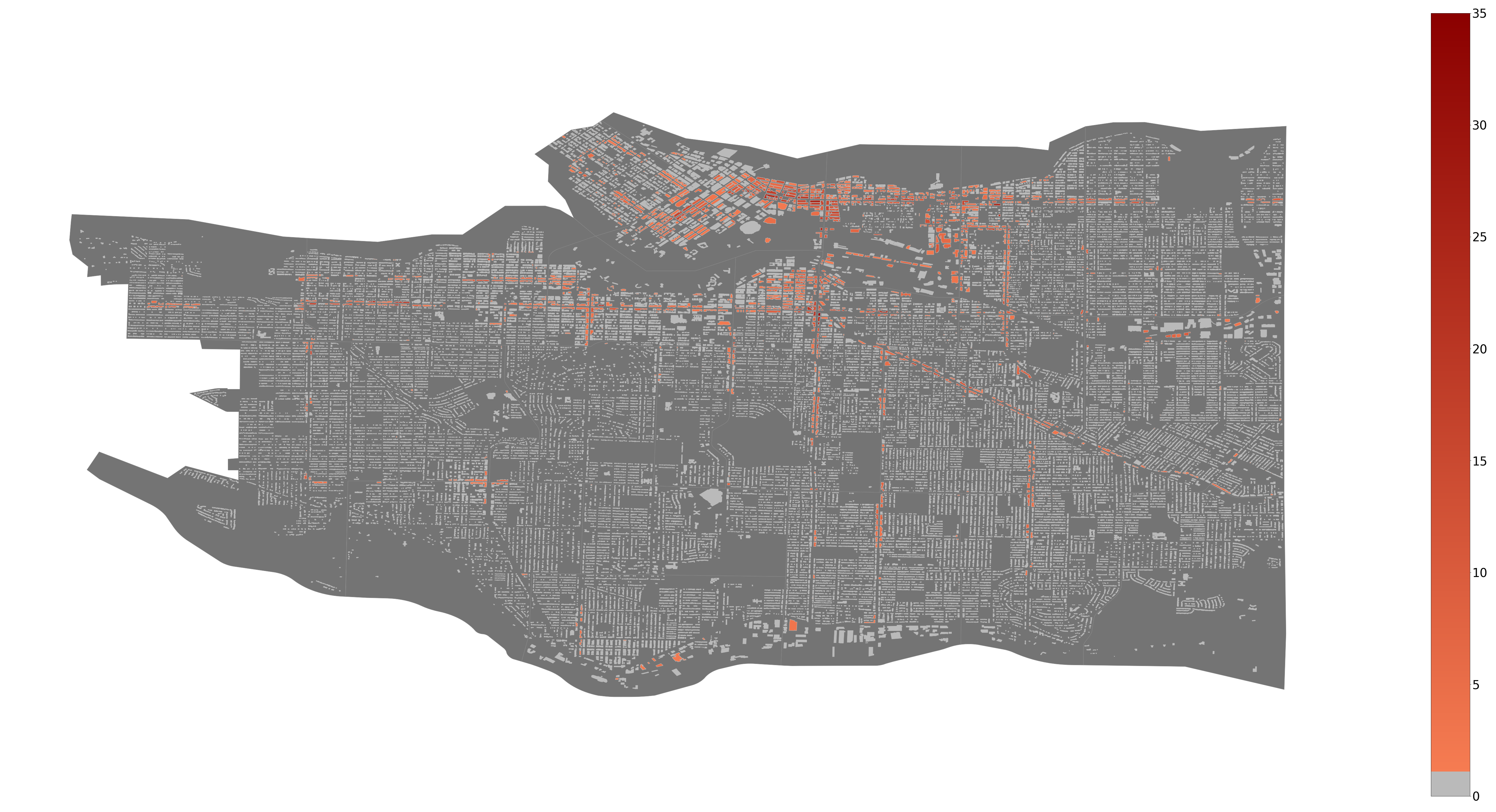
Fig. 3.1. A heatmap of the existing graffiti on each building in Vancouver.
While the Linear Regression gave an R2 score of 0.60 on the test set, the Neural Network gave a score of 0.62, meaning both of these models could explain about 60% of the variance in graffiti counts. However, these include the buildings with 0 graffiti. If we remove these and only consider the vandalized buildings, the R2 of Linear Regression is 0.38, while the Neural Network is 0.41. Therefore, if we were to use these models in another city, we would choose the Neural Network. Fortunately for us, Linear Regression is not so far behind in terms of the score; hence we can use it to explain and highlight the important features which contribute to a building being more or less vandalized.
We use the Linear Regression model to highlight and explain the most contributing features because it is more interpretable than a Neural Network. These features are shown in the following two tables, alongside their importance. The first table shows features which our model has found to deter graffiti. The lower the coefficient, the more they deter. The second table shows which features were found to increase the chances of a building being vandalized. The higher the coefficient, the more it encourages graffiti. In general, a higher absolute value of the coefficient indicates higher importance of the feature. To see the full feature-coefficient table for this model and other models, you may check out our additional statistics page.
| Feature | Coefficient |
| pop_density | -7.68047 |
| street_type_residential | -0.04914 |
| two_houses_away_buildings_average_sub_buildings | -0.04567 |
| one_house_away_buildings_average_height | -0.03249 |
| one_house_away_buildings_count | -0.02273 |
Fig. 3.2. Features which our model has found to deter graffiti.
This table tells us that the higher the population in an area, the less chance of graffiti. Furthermore, buildings on a residential street are less likely to be vandalized. Additionally, more dense areas have an advantage over sparser areas. Higher building density would decrease the probability of an individual building having graffiti. Lastly, tall buildings in the vicinity of a building were also found to deter graffiti.
| Feature | Coefficient |
| one_house_away_graffiti_average | 0.46045 |
| four_houses_away_graffiti_average | 0.31345 |
| two_houses_away_graffiti_average | 0.27223 |
| street_type_arterial | 0.16828 |
| roof_type_Flat | 0.09962 |
Fig. 3.3. Features which our model has found to increase the likelihood of graffiti.
From this table, we learn that more graffiti in the vicinity of a building will increase the chances of that building having graffiti. Buildings on arterial streets and those with flat roof types will also have a higher chance of being vandalized, as was hypothesized in our observations.
From the information in these tables, we learn that, when planning cities, we should have more dense areas and fewer buildings with very few people next to them. Our hypothesis is that if there are more people in an area, there are consequently more eyes protecting it from vandalism. We also learn that graffiti spreads similar to a virus, that is, from one building to the next. Hence, in cleanup operations, buildings at the edge of the ‘infected’ area should be dealt with first, because buildings at the heart of the area have a higher chance of having graffiti put on them again, since they are surrounded by more ‘infected’ buildings than ones at the edges. This could also be explained by people having less hesitation to paint on buildings with existing graffiti than on clean buildings or in an area with less graffiti. Cleaning present graffiti would then prove to be the most effective preventative measure.
Furthermore, we should avoid building on arterial roads or at least invest additional resources for graffiti prevention. We hypothesise that arterial streets have lots of traffic and thus onlookers for the graffiti in case the perpetrator wishes to present a message. Arterial roads are also key avenues of movement and are easily accessible, possibly increasing the risk of graffiti. Lastly, since buildings with a flat roof type attract more graffiti, we should invest in higher quality and more elaborate buildings rather than plain ones. This will be more cost-effective since there will not be any need for cleanups in the long run.
The following map shows the resulting Vancouver graffiti heatmap if nothing is done. This was generated by fitting a linear regression model on the entire dataset and then putting that same dataset through the model.

Fig. 3.4. Logistic Regression predicted heatmap.
Compared to the original heatmap, we notice that graffiti in Downtown, Mount Pleasant, and Westend is set to increase, while the southern part of Marpole is trending towards becoming the newest hub for graffiti. Consequently, it would be a good idea to target these areas when it comes to allocating enforcement.
Classification
Next, we consider the problem of classification, where buildings either have graffiti or do not. This means that we are not concerned with the amount of graffiti the building contains, just if it is clean or if it has been vandalized. The following map indicates buildings with graffiti on them in red.
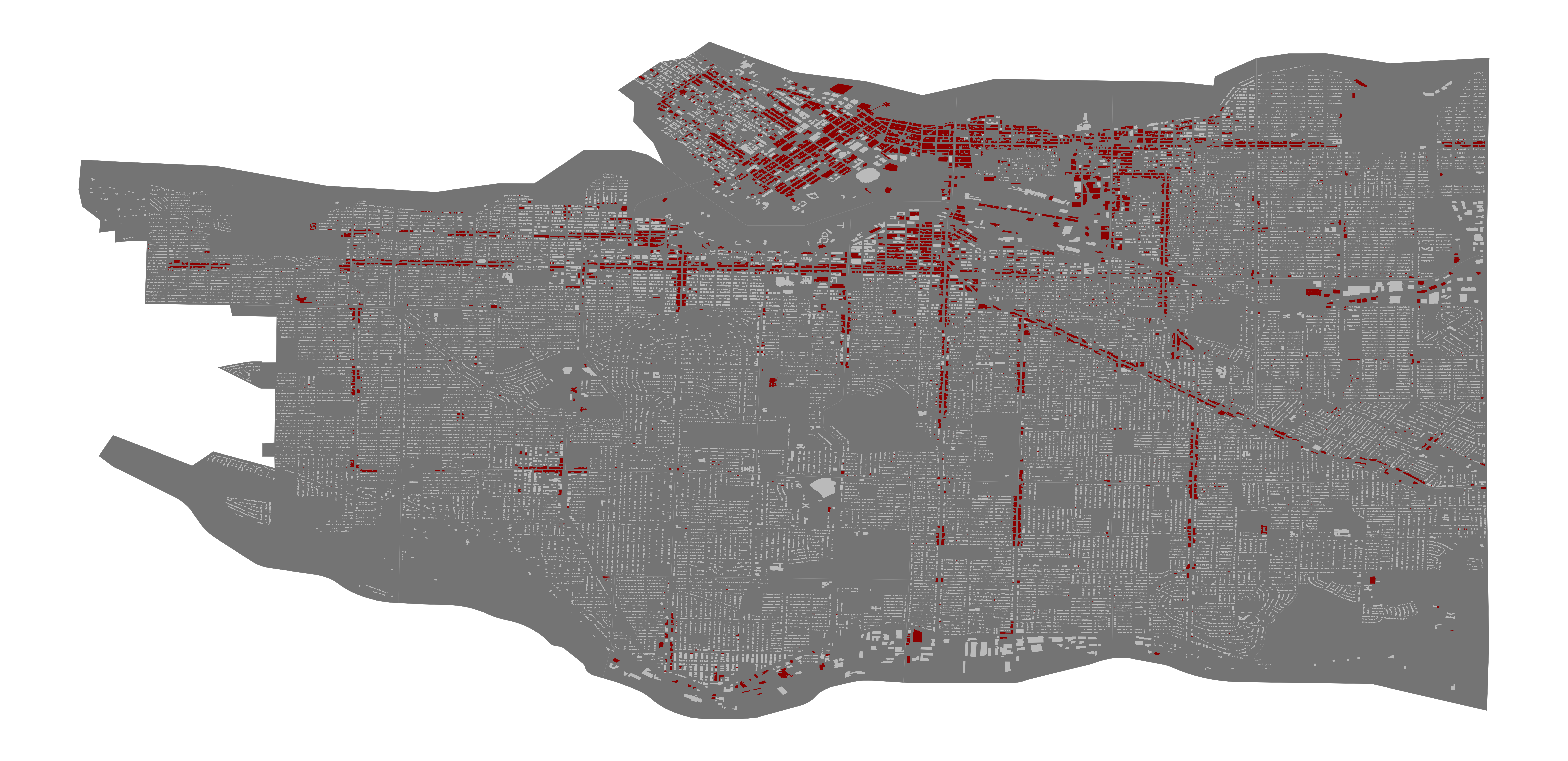
Fig. 3.5. Original classification heatmap.
The following table shows the classification metrics for our classification models. It is important to note that the f1-score is more important than accuracy for our case, since we have an imbalanced dataset.
| - | Logistic Regression | Neural Network | Logistic Regression with Balanced Class Weights |
| accuracy | 0.96 | 0.96 | 0.93 |
| precision | 0.92 | 0.80 | 0.55 |
| recall | 0.63 | 0.65 | 0.84 |
| f1-score | 0.71 | 0.72 | 0.67 |
Fig. 3.6. The classification metrics for our classification models.
As can be seen, the neural network is not drastically more accurate than the basic logistic regression model. Thus, we can use the logistic regression models to explain our data and provide suggestions to mitigate graffiti. We will look at both the normal Logistic Regression models and the one trained with balanced class weights.
Logistic Regression
The following confusion matrix shows the averages of how the logistic regression model classifies the test set.
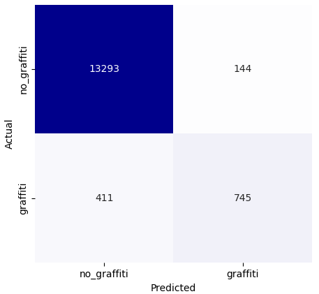
Fig. 3.7. Logistic Regression confusion matrix.
Here, we see that the model does not have many false positives. When it comes to governments allocating enforcement funds, this model is useful for those governments with fewer resources. This is because the model will not waste resources by predicting areas which will not have graffiti as being prone to vandalism. On the other hand, the disadvantage is that it has many more false negatives. Consequently, an area may have graffiti in the future, but the model will not always tell us of it.
To predict, The most important features for this model are listed in the following tables. First, we show those features which prevent graffiti from being put on a building and then those that encourage more graffiti.
| Feature | Coefficient |
| one_house_away_buildings_count | -0.61574 |
| four_houses_away_graffiti_count | -0.48861 |
| one_house_away_graffiti_count | -0.31271 |
| four_houses_away_buildings_average_height | -0.29376 |
| one_house_away_buildings_average_height | -0.28481 |
Fig. 3.8. Features which prevent graffiti from being put on a building
From the above, we see that more nearby buildings will prevent graffiti. Furthermore, if nearby buildings have a large number of graffiti on them, there is less chance that the building in question will have graffiti. Lastly, if the nearby buildings are tall on average, this is also seen to prevent vandalism.
| Feature | Coefficient |
| four_houses_away_graffiti_buildings | 0.82626 |
| one_house_away_graffiti_buildings | 0.77280 |
| one_house_away_buildings_median_height | 0.38123 |
| one_house_away_graffiti_average | 0.34206 |
| four_houses_away_graffiti_average | 0.28826 |
Fig. 3.9. Features which encourage more graffiti.
As we also saw for regression, the more buildings with graffiti near a building, the more chance a building will have graffiti. If the median height of a nearby building is tall, this is shown to increase vandalism. Lastly, if the average number of graffiti on nearby buildings is large, this will increase the probability of the current building in question having graffiti.
In conclusion, the more people occupy nearby buildings, the less vandalism there will be in the area. Analogous observations were made in the regression section. Another similar correlation we find is that if nearby buildings have a lot of graffiti, then so will the other buildings in the area. In spite of this, we notice that if the count of the graffiti of the nearby buildings is high, then there is less chance of the current buildings having graffiti. We form the hypothesis that this is because buildings with high graffiti density act as a ‘magnet’ for new graffiti, protecting other buildings from sharing the same fate.
If we were to use this model for predicting which buildings are going to have graffiti in the future, we end up with this heatmap:

Fig. 3.10. Logistic Regression prediction heatmap.
Logistic Regression with Balanced Weights
In the case of Logistic Regression with the balanced weights, the confusion matrix looks quite different.
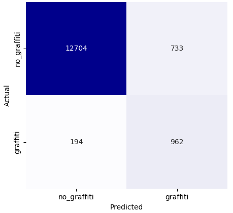
Fig. 3.11. Balanced Logistic Regression confusion matrix.
Here, we see that this model prioritizes avoiding false positives; however, it has more false negatives. As a result, this model may be more beneficial for governments with ample resources in their enforcement department who wish to eradicate graffiti at all costs. Using this model, they will end up putting up enforcement in some areas which may not need it. On the flip side, they will not be missing enforcement in areas which really need it, which is the advantage of this model over the previous Logistic Regression model with imbalanced weights.
As previously done, we also analyze the most important features for this model.
| Feature | Coefficient |
| four_houses_away_graffiti_count | -0.88994 |
| one_house_away_buildings_average_sub_buildings | -0.79784 |
| one_house_away_buildings_count | -0.51494 |
| four_houses_away_buildings_average_height | -0.43637 |
| one_house_away_graffiti_count | -0.32885 |
Fig. 3.12. The most important features for this model.
| Feature | Coefficient |
| four_houses_away_graffiti_buildings | 1.20029 |
| one_house_away_graffiti_buildings | 0.72744 |
| one_house_away_buildings_median_sub_buildings | 0.70437 |
| four_houses_away_graffiti_average | 0.47396 |
| two_houses_away_graffiti_buildings | 0.41469 |
Fig. 3.13. The most important features for this model with a new feature.
Similar to the previous models, the same features contribute to the probability of a building having more or less graffiti. The one interesting new feature is that a high average of nearby sub buildings will decrease the chance of graffiti, while a high median will increase it.
When used to predict new graffiti, this model produced the following result. As discussed in the confusion matrix, one can notice how it predicts more graffiti than the previous model. Similar to how the regression model predicted, the southern part of Vancouver is prone to becoming a hub for graffiti, and so is the upper-middle Eastern part.
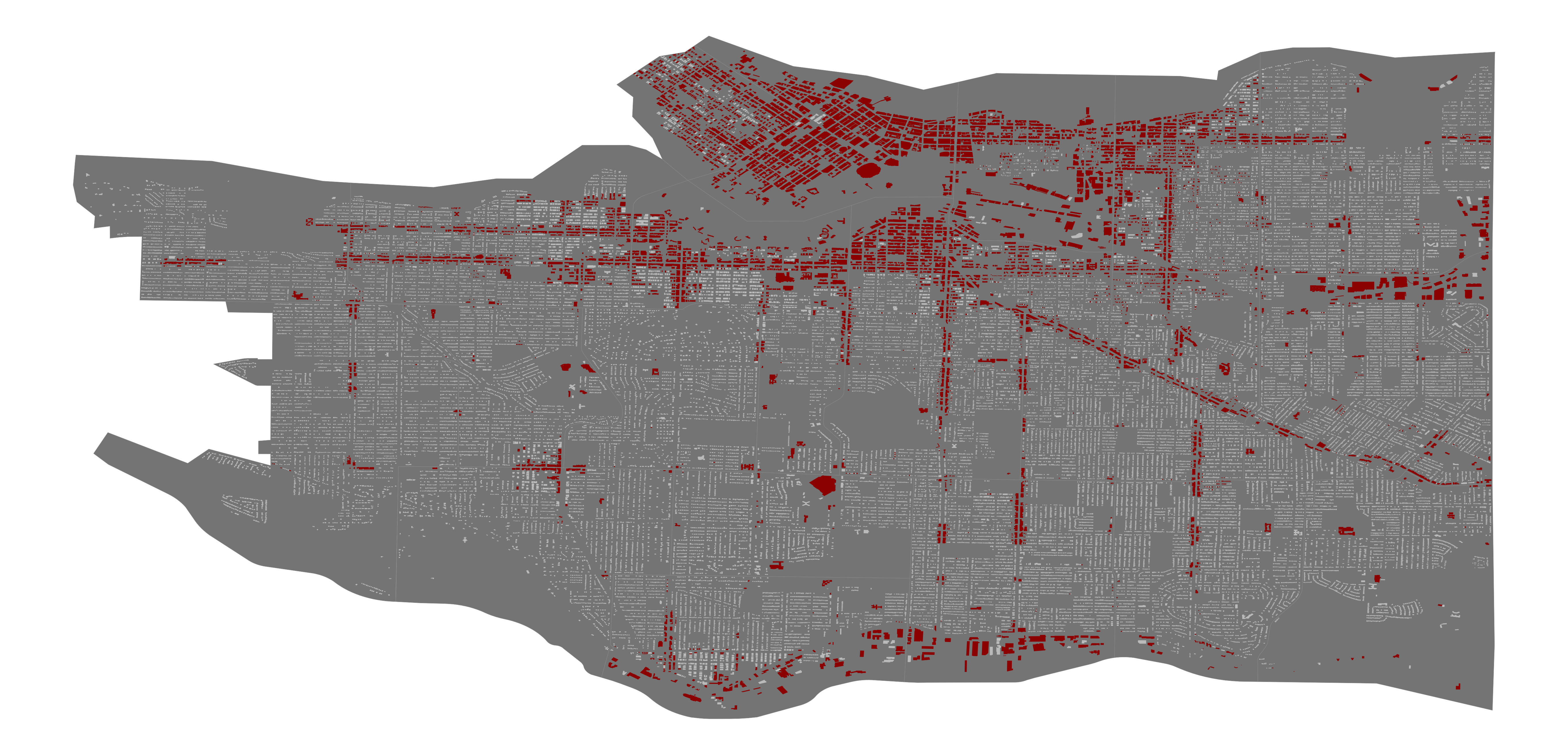
Fig. 3.14. Balanced Logistic Regression prediction heatmap.